
Some clear and not too surprising trends emerge from our survey of the biomes of the world in terms of what controls their productivity and and growth.
First, and foremost, productivity is strongly correlated with precipitation
and temperature. Some researchers combine these two variables into one
single parameter, actual evapotranspiration, or AET. The figure shown below
shows the strong relationship between AET and total above-ground production
for several sites around the world. We can also find relationships between
above-ground biomass in terrestrial systems and AET and production.

Whittaker (his Figure 4.10 in his book) shows a diagram of the major biomes as plotted against both mean annual precipitation and mean annual temperature. Thus, areas with low precipitationl, and cold temperatures fall out as alpine or tundra systems. There are no systems known where there is abundant precipitation coupled with very low temperatures.

If precipitation stays low, but temperatures moderate some, then there is a transition to taiga and boreal forests. Further warming leads us through savannas, grasslands, and at the warmest end of the spectrum to thorn scrublands and savanna woodlands.
If we follow warm temperatures across the moisture gradient, from least to most, then we make the transition from deserts with little or no moisture, to tropical seasonal forests, to rainforests at the upper end of the precipitation range. At moderate temperatures, and moderate to high precipitation, we find temperate forests and temperate rainforests.
Other unique combinations can be found if the seasonality of the precipitation is brought into this scheme, for example, at moderate temperatures and low rainfall, but with the rainfall concentrated in the winter season, you get Mediterranean or chaparral systems, common along the west coast of the United States and the Mediterranean Sea.
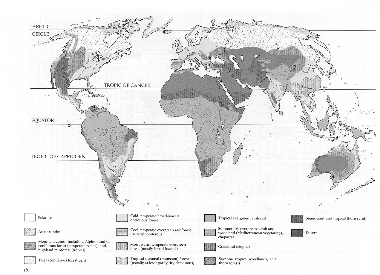
The figure below shows the world's biomes:
To see global patterns of NPP, and other associated variables to drive models that map these patterns, go to the web site shown below:
http://www.inform.umd.edu/Geography/glopem/
This is from the University of Maryland's Global Research Program.
Each year, the earth receives 55 kCal cm-2 in the visible range. This is not evenly distributed over the surface of the earth (more is received in the tropics than at the poles, more where there are fewer clouds). How the biota use this radiation is of interest, because sunlight is ultimately the main source of energy for most of the world's ecosystems (excluding perhaps communities deep within the ocean near thermal vents, which depend on sulfur compounds for energy).
Primary production is the rate at which energy is bound, or organic material is created by photosynthesis, per unit of the earth's surface per unit time (Whittaker, 1975, pg. 193). It is a rate, not an amount! It is often expressed as g m-2 yr-1, or in energetic terms, as kCal m-2 yr-1. We should take care to distinguish between production, which is a rate, and the amount of biomass at any one time, which is referred to as the standing crop (g/m2, or t/ha).
The total amount of energy bound by photosynthesis (we refer here mainly to terrestrial systems, but this also applies to aquatic ones too) or the amount of organic matter created, is known as gross production. The amount of organic material left after respiration by plants is the net primary productivity (known as NPP). Because plants produce their own organic matter, they are known as autotrophs. It is only this latter amount that is available to other organisms for consumption or use. Productivities of animals and saprobes (known as heterotrophs) is secondary productivity.
How Production is Measured
The simplest way to measure productivity in terrestrial systems is
to conduct periodic harvests throughout the growing season. The harvests
should not be spread too far apart, or you can miss production that is
consumed by insects and other organisms, or that is produced, but which
senesces before you come back to take a second measurement. Large
numbers of plots usually need to be measured, because of high variability
in natural systems. Harvests done only at the end of a season usually
underestimate the actual NPP.
Belowground measurement of NPP is very complicated, due to the difficulty of harvesting roots, the spatial variation, and the technical problems with knowing how often to harvest. Root turnover, which is a measure of how often new roots are produced, can lead to serious underestimates of actual productivity occurring belowground. Besides measuring rates, even determining the standing crop of belowground biomass is extraordinarily difficult. One book on root techniques even suggested that to get the entire root system out of the ground for weighing purposes, one should consider using dynamite. The author cautioned though, that this technique might result in the loss of some of the fine roots!
Measuring gross productivities can be difficult also, since you have to know respiration rates, rates of photosynthesis, and so on. We won't deal with this in this course.
If one wants to measure the NPP of natural forest systems, though, other techniques need to be adopted. Whittaker pioneered the use of allometric equations to estimate NPP. He called his technique dimension analysis. Here is the schema for how to do this (Whittaker, 1975, pg. 194):
1. Trees in sample quadrats
are measured for diameter at the base and breast height.
2. A set of sample trees
is cut and subjected to detailed analysis - one determines the dry weights
of leaves, branches,
bole, and roots if possible, and other fractions, such as flowers and fruits.
By looking at ring widths of the bole
and branches, estimates of NPP are obtained.
3. Then, logarithmic equations
are developed which relate biomass and production estimates to diameter
at breast or bole
height. This is done for each biomass fraction.
4. The equations are used
to estimate NPP for each tree species, and then summed for all trees within
a quadrat. These
values are then extrapolated for the entire forest stand or ecosystem.
Typical NPPs for temperate forests average around 1200 g m-2
yr-1. Mature forests have a larger fraction of their
biomass in stems, and smaller fractions in branches and leaves. Nearly
40-60% of standing biomass may be underground!
If you measure photosynthesis and respiration of plants, you can make estimates of their gross production:
Gross Production = NPP + Respiratory Losses
In temperate forests, measurements indicate that nearly 55% of the gross production is consumed by respiration, leaving only 45% available for harvest by animals or decomposers.
In a forest on Long Island, near Brookhaven, NY, Whittaker estimated that about 8% of the leaf weight is consumed by insects each year. Since leaves make up 33% of the total NPP, then 8% consumed is only 0.08*0.33 = 2.6% of the total NPP. In other forests, herbivores may consume anywhere from 1% or less to over 7% (values may be higher in Australia, for reasons we'll discuss later in the course). How much belowground material is consumed varies considerably, and that too will be discussed later on, but suffice it to say, that it is more than you might think!
The accumulation of biomass in an ecosystem depends on the difference between gross productivity and total community respiration. This is termed net ecosystem production, and is not the same as NPP. For example, in a mature forest, NPP may be quite high (over 1200 g m-2 yr-1) but net ecosystem production may be near zero, because gross production is nearly balanced by respiration of all organisms in the community. In late stage forests, where there is less leaf material relative to woody material, there is less photosynthesis, but a lot more respiration, especially from the branches and boles and roots, which may completely counter any gains from net carbon uptake by photosynthesis. As one moves to warmer and wetter areas, which stimulate respiration, the percentage of gross productivity used up in respiration increases. Tropical rainforests have very high respiration rates, and large differences between gross and net primary productivity.
Animal Secondary Productivity
For animals, measuring secondary productivities can be difficult.
Whittaker (1975, pg. 199) defines secondary animal productivity as:
"the formation of new protoplasm by heterotroph populations, as measured
in dry grams
or organic matter (or equivalent energy) per unit area and time."
As an example of the difficulty, consider that even though animals may eat 8% of the leaves in the Brookhaven Forest on Long Island, not all of that is turned into secondary animal productivity. There is some fraction that is indigestible, some is given off as respiration, some is incompletely digested. In caterpillars, some 80-90% of the leaf material ingested is passed through the gut without being absorbed or digested! The main relationships are:
Ingestion = Assimilation + Egestion
Assimilation is used for respiration and productivity
Productivity is used for growth and reproduction
In animal populations, the above relationships must be known for all age classes, and through the season. This makes it very difficult to quantify on large populations in the field. Consider this example from Whittaker, pg. 200:
Supppose you have a grasshopper
population with a density of 3 individuals/m2. Each grasshopper
weighs 67 mg, and therefore, in one square meter you have 200 mg of grasshopper.
From laboratory measurements, we know that one grasshopper eats 0.28 g
of grass per gram body dry weight per day. 62% of food eaten is egested,
and 38% assimilated. Of this latter amount, 34% is respired away,
and only 4% becomes secondary productivity.
The population's productivity is 200 mg X 0.28 X
0.04 = 2.2 mg m-2 day-1. Summing
up over the season, and incorporating variation in grasshopper size, scientists
estimated that on an annual basis total assimilation was 1.1 g m-2
yr-1 and secondary production was 0.12 g m-2 yr-1.
When all arthropods were summed, it was found that they consumed 10.6%
of the aboveground NPP.
Determinants of NPP in Communities Worldwide
Whittaker (1975, pp. 202-205) provides a succinct discussion of the
factors affecting NPP in communities around the world. As one moves
from very dry areas to wetter ones, there is a nearly linear relationship
between NPP and rainfall, at least below 500 mm/yr. See the figure
below. Beyond 500 mm/yr, other factors begin to become important.
Figure 2.4 in the beginning of this lecture shows the strong relationship
between NPP and evapotranspiration. For temperature, the relationship
is curvilinear, rising sharply at mid-range temperatures, but moving more
slowly at very cold temps, and very hot temps (See Figure 5.4, from Whittaker,
1975). At the highest ranges, tropical rainforests, marshes, and
agricultural fields (sugar cane and rice) productivities may be 3,000 g
m-2 yr-1 . As temperatures are lowered, NPPs
go down, although there is a lot of scatter in the data (high variability
due to other factors besides temperature).
One can also express the ratio of biomass to productivity, which is
known as the biomass accumulation ratio. This ranges from 2-10 in
deserts (aboveground biomass only), 1-3 in grasslands, 3-12 in shrublands,
and 10-30 in woodlands up to a maximum of 20-50 in mature forests.
Although we might suspect that NPP can be greatly increased in terrestrial
systems, the fact that they are still low in the natural world suggests
that other factors are limiting NPP, such as nutrient deficiencies, water
limitations, etc. To significantly raise NPPs would require substantial
intervention on the part of humans, in the form of fertilizers, water,
and so on. This can only be done in most cases at high cost to society,
which in turn, suggests that large increases in NPP to serve human needs
will not come easily, if at all.
Bray, J.R. and E. Gorham. 1964. Litter production in forests of the world. Advances in Ecological Research 2:101-157.
Cramer, W., D.W. Kicklighter, A. Bondeau, B. Moore III et al.
1999. Comparing global models of terrestrial net primary
productivity (NPP): an overview.
Global Change Biology 5: 1-15.
Lieth, H. and R.H. Whittaker, editors. 1975. The Primary Production of the Biosphere. Springer Publishers, NY.
Newbould, P.J. 1967. Methods for estimating the primary production
of forests. International Biological Programme
Handbook 2, viii
+ 62 pp. Blackwell Scientific Publ., Oxford.
Phillipson, John. 1966. Ecological Energetics. Arnold Publishers. 57 pp.
Schimel, D.S. 1995. Terrestrial ecosystems and the carbon cycle. Global Change Biology 1:77-91.
Schimel, D.S. 1995. Terrestrial Biogeochemical cycles: Global
estimates with remote sensing. ISLSCP Special Issue of
Remote Sensing of Environment 51:49-56.
Schimel, D.S., B.H. Braswell, E.A. Holland, R. McKeown, D.S. Ojima,
T.H. Painter, W.J. Parton, A.R. Townsend. 1994. Climatic, edaphic and
biotic controls over storage and turnover of carbon in soils. Global
Biogeochemical Cycles
8(3):279-293.
Smalley, A.E. 1960. Energy flow of a salt marsh grasshopper population. Ecology 41:672-677.
Van Hook, R.I. 1971. Energy and nutrient dynamics of spider and
orthopteran populations in a grassland ecosystem.
Ecological Monographs
41:1-26.
Whittaker, R.H. 1975. Communities and Ecosystems. MacMillan
Publishers, NY, NY. 385 pp.
Note: This book contains many useful figures
and references on production and NPP.
Whittaker, R.H. and G.M. Woodwell. 1968. Dimension and production
relations of trees and shrubs in the Brookhaven
Forest, New York. Journal
of Ecology 56:1-25.
Whittaker, R.H. and G.M. Woodwell. 1969. Structure, production
and diversity of the oak-pine forests at Brookhaven,
New York. Journal of
Ecology 57:157-174.